nextnano³ - Tutorial

next generation 3D nano device simulator

2D Tutorial

Landau levels of a bulk GaAs sample in a magnetic field

Note: This tutorial's copyright is owned by Stefan Birner, www.nextnano.de.

Author: Stefan Birner

If you want to obtain the input files that are used within this tutorial, please contact stefan.birner@nextnano.de.
 -> 2DBulkGaAs_LandauLevels.in
 

Landau levels of a bulk GaAs sample in a magnetic field

In this tutorial we study the electron energy levels of a bulk GaAs sample that is subject to a magnetic field.

• The GaAs sample extends in the x and y directions (i.e. this is a two-dimensional simulation) and has the size of 300 nm x 300 nm.
  At the domain boundaries we employ Dirichlet boundary conditions to the Schrödinger equation, i.e. infinite barriers.
   
• The magnetic field is oriented along the z direction, i.e. it it perpendicular to the simulation plane which is oriented in the (x,y) plane).
  We calculate the eigenstates for different magnetic field strengths (1 T, 2 T, 3 T), i.e. we make use of the magnetic field sweep.
  
    $magnetic-field
   magnetic-field-on                    = yes
   magnetic-field-strength              = 1.0d0   ! 1 Tesla = 1 Vs/m²
   magnetic-field-direction             = 0 0 1   ! [001] direction
   magnetic-field-sweep-active          = yes     !
   magnetic-field-sweep-step-size       = 1.0d0   ! 1 Tesla = 1 Vs/m²
   magnetic-field-sweep-number-of-steps = 2       ! 2 magnetic field sweep steps
  $end_magnetic-field
   
• A useful quantitiy is the magnetic length (or Landau magnetic length) which is defined as:
      l_B = [h_bar / (m_e* w_c)]^1/2 = [h_bar / (|e| B)]^1/2
  It is independent of the mass of the particle and depends only on the magnetic field strength:
  - 1 T: 25.6556 nm
  - 2 T: 18.1413 nm
  - 3 T: 14.8123 nm
   
• The electron effective mass in GaAs is m_e* = 0.067 m₀. Another useful quantity is the cyclotron frequency:
      w_c = |e| B / m_e*
  Thus for the electrons in GaAs, it holds for the different magnetic field strengths:
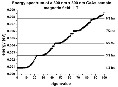
  - 1 T: h_barw_c = 1.7279 meV
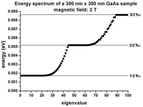
  - 2 T: h_barw_c = 3.4558 meV
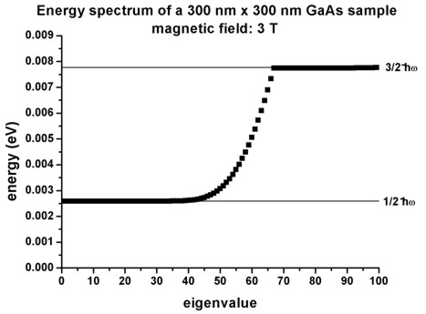
  - 3 T: h_barw_c = 5.1836 meV

• The energy spectra for different magnetic fields (1 T, 2 T, 3 T) look as follows:
   

• The Landau levels are given by E_n = (n - 1/2) h_barw_c where n = 1,2,3,...
   
• The number of states for each Landau level can be calculated as follows (see P.Y. Yu, M. Cardona, Fundamentals of Semiconductors, p. 536, 3^rd ed.):
      N = L_xL_y |e| B / h = 1/(2pi)  L_xL_y / l_B²        (ignoring spin)
  where L_x and L_y are the lengths in the x and y directions (300 nm in this example) and l_B is the magnetic length.
  
  N(1 T) = 21.76 ==> ~22 states per Landau level (in the figure above: 22 as it should be)
  N(2 T) = 43.52 ==> ~44 states per Landau level (in the figure above: 44 as it should be)
  N(3 T) = 65.29 ==> ~66 states per Landau level (in the figure above: 66 as it should be)
  
  Note that N is independent of n.
• For the calculations, we used the symmetric gauge A = - 1/2 r x B = 1/2 B x r
  leading to the following energies (see J.H. Davies, The Physics of Low-Dimensional Semiconductors, p. 222):
      E_n,l = (n + 1/2 l + 1/2 |l| - 1/2) h_barw_c
  One can see that all states having a negative value of 'l' are degenerate with the states with l=0, i.e. the allowed energies are independent of l if l < 0 (for the same n).
  The energies increase if l increases (for l > 0 and for the same n).
   
• The motion in the z direction is not influenced by the magnetic field and is thus that of a free particle with energies and wave functions given by:
     E_z = h_bar² k_z² / (2 m*)
     psi(z) = exp (+- i k_z z)
  For that reason, we did not include the z direction into our simulation domain, and thus only simulate in the (x,y) plane (two-dimensional simulation).

• Please help us to improve our tutorial. Send comments to support [at] nextnano.de.