Database
Effective masses
 conduction-band-masses    =
  m    m
m       !
Gamma valley (m,m,m)
ml,L mt,L mt,L !
ml,X mt,X mt,X !
1/m are the masses in the principal axes system of the minima.
These masses are associated to the eigenvectors of the minima in the order they
are given in the parameter set. The eigenvectors are specified by their
coordinates in the cartesian coordinate system of the crystal.valence-band-masses
Conduction band masses
We have to specify 9 values for the conduction band masses. For each valley
(Gamma, L, X) we have one line and for each valley we need to specify the
longitudinal (ml) and the transverse masses (mt1,mt2)
where mt1=mt2=mt.
e.g. GaAs
1st      2nd      3rd
principal axis
 conduction-band-masses    = 0.067d0  0.067d0
0.067d0  !
Gamma valley (m,m,m)
1.9d0 0.075d0 0.075d0 !
1.98d0 0.27d0 0.27d0 !
The order is important for the L and X valleys (mlongitudinal, mtransverse,
mtransverse).
 conduction-band-masses    = m    m
m       !
Gamma valley (m,m,m)
ml,L mt,L mt,L !
ml,X mt,X mt,X !
These masses represent a mass tensor (1/m)ij given in the principal-axes system:
  1/m     0      0
!
Gamma valley
   0     1/m     0    !

   0      0     1/m   !
  1/ml,L   0      0
!
L valley
   0     1/mt,L   0    !

   0      0     1/mt,L !
  1/ml,X   0      0
!
X valley
   0     1/mt,X   0    !

   0      0     1/mt,X !
|
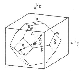 
This picture shows the first Brillouin zone
for zinc blende and diamond structure crystals (left) and for wurtzite
(right).
Constant-energy surfaces characterizing the conduction-band-structure in
(a,d) Ge, (b) Si, and (c) GaAs.
(d) shows the truncation of the Ge surfaces at the Brillouin-zone
boundaries. |
The degeneracy of the Gamma valley is 1, of the L valley it is 8 and of the X
valley it is 6. The L and X valleys are shared with the adjacent first Brillouin
zone thus we take only half the value:
conduction-band-degeneracies = 2 8 6 ! (including spin
degeneracy)
number-of-minima-of-cband = 1 4 3
In the case of Si, where the X valleys lie completely inside the first
Brillouin zone, we take twice as much as the conduction band degeneracy for its
valleys. The degeneracy includes the number of degenerate minima per band as well as
the twofold spin-degeneracy.
conduction-band-degeneracies = 2 8 12 ! (including spin
degeneracy)
number-of-minima-of-cband = 1 4 6 !
Now we have to specify, where these minima are located in the crystal-axes
system (components of k vector along crystal xyz [k0]). The position of the minima in k-space is defined
by the specifier conduction-band-minima. The coordinates are in units of [2pi/a]
within the crystal
coordinate system where a is the lattice constant.
Note: Currently it is assumed in parts of the program, that the ordering
of the conduction band minima is like
1=Gamma (zone center),
2=L (along <111> direction),
3=X (along <100> direction).
conduction-band-minima = v11 v12 v13
v21 v22 v23
v31 v32 v33
...
k vectors to individual conduction band minima.
As many vectors (coordinate triplets in crystal coordinate system) as individual
minima.
Let's assume we have 3 conduction band minima 1,2,3 as specified above.
These minima are deg1,deg2,deg3-fold degenerate. In this case,
input for deg1/2+deg2/2+deg3/2 vectors has to be provided. The
factor 1/2 is due to spin degeneracy which is already included in the degeneracy
factors.
GaAs:
 conduction-band-minima =
0d0
0d0      0d0     ! Gamma


!


0.866d0  0.866d0  0.866d0 ! L1  1 1 1


0.866d0  0.866d0 -0.866d0 ! L2  1 1-1


-0.866d0  0.866d0  0.866d0 ! L3 -1 1 1


-0.866d0  0.866d0 -0.866d0 ! L4 -1 1-1


!


1d0      0d0      0d0      ! X1  1 0 0


0d0      1d0      0d0      ! X2  0 1 0


0d0      0d0
1d0      ! X3  0 0 1
(We have to specify only half the amount of the L and X minima (namely 4
instead of 8 (L) and 3 instead of 6 (X)). For Si we have to specify 6 X valleys
as they lie completely inside the first Brillouin zone.
(The value of 0.866 is due to 31/2/2 = 0.866025.)
Si: (X valley minimum at e.g. at k=(0.85,0,0)
[2pi/a] where a is the lattice constant.)
 conduction-band-minima =
0d0
0d0      0d0      ! Gamma


!


0.866d0  0.866d0  0.866d0 ! L1   1 1 1


0.866d0  0.866d0 -0.866d0 ! L2   1 1-1


-0.866d0  0.866d0  0.866d0 ! L3  -1 1 1


-0.866d0  0.866d0 -0.866d0 ! L4  -1 1-1


!


0.850d0  0d0      0d0     ! X1   1 0 0


0d0      0.850d0  0d0      ! X2   0 1 0


0d0      0d0      0.850d0 ! X3   0 0 1


-0.850d0  0d0      0d0     ! X4  -1 0 0


0d0     -0.850d0  0d0      ! X5   0-1 0


0d0      0d0     -0.850d0 ! X6   0 0-1
As we specify the effective masses (ml, mt, mt) in the principal-axes system,
i.e. (1/ml, 1/mt, 1/mt), we have to
specify some rotation matrices to project the masses of the principal-axes
system into the appropriate directions inside the crystal-axes system.
For this we specify for each Gamma, L and X valley its principal-axes
system.
The effective masses are defined in the principal-axes
system of the minima (principal-axes-cb-masses). These masses are
associated to the eigenvectors of the minima in the order they are given in
the parameter set. The eigenvectors are specified by their coordinates in the
cartesian coordinate system of the crystal.
The units are not important because only the direction is.
The normalization will be done internally by the program in
SUBROUTINE
normalize_principal_axes
.
principal-axes-cb-masses = a11 a12 a13
b11 b12 b13
c11 c12 c13
    ....


....


....


     a21 a22 a23
b21 b22 b23
c21 c22 c23
       ....


....


....


       a31 a32 a33
b31 b32 b33
c31 c32 c33
      ....


....


....
Completely analog as conduction-band-minima, but this time 3 vectors
for each individual minimum. The orderering of the principal axes is associated
to the ordering of the conduction-band-masses.
principal-axes-cb-masses
= 1d0      0d0      0d0     ! Gamma


0d0      1d0      0d0


0d0      0d0      1d0
1d0      1d0
1d0      ! L1


1d0     -1d0      0d0


1d0      1d0     -2d0


1d0      1d0     -1d0      ! L2


1d0     -1d0      0d0


-1d0     -1d0     -2d0


-1d0      1d0      1d0      ! L3


1d0      1d0      0d0


-1d0      1d0     -2d0


-1d0      1d0     -1d0      ! L4


1d0      1d0      0d0


1d0     -1d0     -2d0
1d0      0d0      0d0      ! X1


0d0      1d0      0d0


0d0      0d0      1d0


0d0     -1d0      0d0      ! X2


0d0      0d0
-1d0


1d0      0d0      0d0


0d0      0d0      1d0      ! X3


1d0      0d0      0d0


0d0      1d0      0d0
The Gamma case is trivial. (We specified the identity matrix and all the
masses have the same value anyway.)
The X case is not difficult either. The multiplication will be done the following way:
AT.M.A where
     1/ml,X    0
0

M =   0      1/mt,X   0

      0       0     1/mt,X
A
is a rotation matrix given for the X1, X2 and X3 minimum (which position
in k space was already defined by the specifier
conduction-band-minima and can be found under the specifier principal-axes-cb-masses, e.g.
for X2:
      0   -1
0

A =   0    0   -1

      1    0
0
A=cb_trans_matrix_mass(mat_num,band_num,min,alloyc)
MCxyz =ATMp-axis A
A ... transformation matrix
MCxyz ... mass tensor in cartesian
crystal coordinate system
Mp-axis ... mass
tensor in principal axis system
For our example for X2 we get
       1/mt,X    0
0

M
Cxyz = 0 1/ml,X 0
0 0
1/mt,X
Then the vectors specified for the X valleys under keyword
conduction-band-minima will be multiplied in the following way:
xT.MCxyz.x=1/ml
Consider again our example:
0d0      1d0      0d0
  ! X2  0 1 0
1/mt,X   0      0

(0,1,0)
T . 0
1/ml,X 0
. (0,1,0) = 1/ml,X
0 0 1/mt,X
As expected, the longitudinal mass points into the direction of the valley.
Similar for the L valley:
Please have a look at this pdf if
you want more details.
The following routines are involved:
FUNCTION
cb_masses
FUNCTION
cb_masses_xyz
FUNCTION
cb_inv_masses_xyz
SUBROUTINE
normalize_principal_axes
Valence bands
They are easier:
valence-band-degeneracies      =
2
2       2      !
including spin degeneracy
valence-band-masses
= 0.79d0  0.79d0  0.79d0 !
heavy hole (hh)
0.14d0 0.14d0 0.14d0 !
0.25d0 0.25d0 0.25d0 !
number-of-minima-of-vband      =
1
1       1      !
valence-band-minima
= 0d0     0d0
0d0     !
hh
0d0     0d0
0d0      !
0d0     0d0
0d0      !
principal-axes-vb-masses       =
1d0
0d0     0d0      !
hh
0d0     1d0     0d0      !


0d0     0d0
1d0      !


1d0     0d0     0d0      !
0d0     1d0     0d0      !


0d0     0d0
1d0      !


1d0     0d0     0d0      !
0d0     1d0     0d0      !


0d0     0d0
1d0      !
Effective mass for density of states calculation
For a single band minimum described by a longitudinal mass (ml)
and two transverse masses (mt) the effective mass for the density
of states calculations is the geometric mean of the three masses.
Effective mass for the density of states in one valley of conduction band:
me*DOS = (ml·mt·mt)1/3
= (ml·mt2)1/3
For instance electrons in the Delta (close to X) minima of Si have an effective DOS mass given
by:
me*DOS = (0.916·0.192)1/3
m0 = 0.321m0
Effective mass for conductivity calculations
The effective mass for conductivity calculations is the mass, which is
used in conduction related problems accounting for the detailed structure of the
semiconductor. These calculations include mobility and diffusion constants
calculations.
As the conductivity of a material is inversionally proportional to the
effective masses, one finds that the conductivity due to the multiple band
maxima or minima is proportional to the sum of the inverse of the individual
masses, multiplied by the density of carriers in each band, as each maximum or
minimum adds to the overall conductivity. For anisotropic minima containing one
longitudinal (ml) and two transverse effective masses (mt)
one has to sum over the effective masses in the different minima along the
equivalent directions. The resulting effective mass for bands, which have
ellipsoidal constant energy surfaces, is given by:
me*cond = 3 / (ml-1
+ mt-1 + mt-1) = 3 / (ml-1
+ 2mt-1)
provided the material has an isotropic conductivity as is the case for cubic
materials. For instance electrons in the X minima of Si have an effective
conductivity mass given by
me*cond = 3 / (1/0.916 + 2/0.19) m0 =
0.258 m0
Note: Holes
Due to the fact that the heavy, light and split-off hole bands do not have a
spherical symmetry there is a discrepancy between the actual effective mass for
the density of states and conductivity calculations and the calculated value
which is based on spherical constant-energy surfaces. The actual constant-energy
surfaces of the e.g. heavy hole band are "warped spheres", resembling a cube with
rounded corners and dented-in faces. This warping is a direct consequence of the
cubic crystal system.
1D
Here, we have one mass in quantization direction and one mass perpendicular
to it.
Description of MODULE
input_quantummodels:
Mass in quantization direction
FUNCTION mass_out_of_plane
Provides out-of-plane mass in quantization direction, m_perpendicular.
e.g. quantization direction = x axis
(1)    / ( m11-1  m12-1  m13-1
)   (1) \    (1)   (m11-1)

    1/m_perp = (0) . (  ( m21-1  m22-1
m23-1 ) . (0)  ) = (0) . (m21-1) = m11-1


(0)    \ ( m31-1  m32-1  m33-1
)   (0) /    (0)   (m31-1)
i.e. quantization direction = x axis -> m_perp = m11 ,
s -> = m22
,
 ->        = m33


 m_perpV(i,j) = 1.0 / DOT_PRODUCT(quantization_directionV(1:3),


(MATMUL(imassM,quantization_directionV(1:3))))
Mass in parallel direction
FUNCTION Get_mass_parallel
Provides averaged mass in parallel direction (in-plane mass). Makes only sense for 1D (and
2D).
Input is effective mass tensor in 1/mij notation.
Output is parallel effective mass (scalar).
Takes 1/mii and 1/mjj and 1/mij=1/mji.
Considers 2x2 matrix and diagonalizes it.
In 1D when we calculate density of states, we generally consider m||=sqrt(m1,||*m2,||).
When everything is symmetric it makes no problem. But when we have a strange
symmetry with off-diagonal elements we have to define a cross-section of the 1/m
ellipsoid and look for its own principal axis. This will be described in the
following.
Here we only consider the relevant 2x2 matrix of the 3x3 mass tensor and
diagonalize it.
We follow Eq. (13) of F. Stern, W. E. Howard, Phys. Rev. 163, 816
(1967) who derived how the in-plane energy dispersion for each subband n, En(k1,k2),
is defined.
It is important to consider the Stern/Howard formula for the L valley (even for
[001] growth) and for the X valleys for non-[001] growth directions.
 matrixM(1,1) = ( w_11 - w_13^2      / w_33 )

 matrixM(2,2) = ( w_22 - w_23^2      / w_33 )

 matrixM(1,2) = ( w_12 - w_13 * w_23 / w_33 )
   = matrixM(2,1)


 ( 1/m_ii   1/m_ij )   ( A   C )

 (
) = (       )

 ( 1/m_ji   1/m_jj )   ( C   B )
Eigenvalues: (A-l)(B-l) - C^2 = 0
-> l^2 - l(A+B) + AB - C^2 = 0
The Mathematica command at www.wolframalpha.com to calculate the eigenvalues, "eigenvalues[{{A,C},{C,B}}]", leads to the following equation:
l_1 = 0.5 * ( A+B + SQRT( A^2 + B^2 - 2AB + 4C^2 ) )

l_2 = 0.5 * ( A+B - SQRT( A^2 + B^2 - 2AB + 4C^2 ) )


discriminant = SQRT( (A-B)^2 + 4C^2 )


imassesV(1) = 0.5 * ( A+B + discriminant )

imassesV(2) = 0.5 * ( A+B - discriminant )


!
imass_out = SQRT( imassesV(1) * imassesV(2) )

 mass_out = 1 / imass_out
Note: This function is also used when one wants to get the degeneracy
of the Schrödinger equations because of different masses in subroutine
get_deg_schroedinger_el1D (splitting of bands due to strain).
|